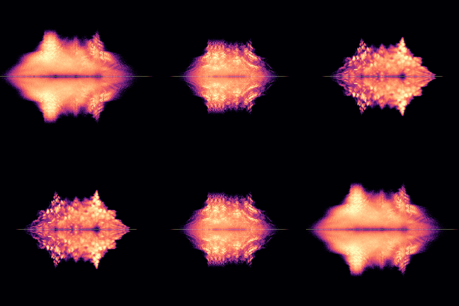
Bohemian eigenvalue explorer

Let $P \subset \mathbb{C}$ be a finite set. Usually $P \subset \mathbb{Z}$, for example $P = \{-1, 0, 1\}$. The Bohemian family of dimension $n$ over $P$ is

Nearly always, a constraint on the set of matrices is added, so the family is limited to $\mathcal{B}_n(P) \cap S$, where $S$ is the set of tridiagonal, Toeplitz, or Hessenberg shaped matrices. These sets exhibit a way to visualise the spectra of finite matrices in a quite trippy way:

1. Pick $n$, a shape $S$, and a value of $t$.
2. Define $P_t = \{-1,\, t,\, 1\}$. At $t = 0$ this is $\{-1,0,1\}$; at $t = \pm 1$ it collapses to two elements. Draw $A$ uniformly at random from $\mathcal{B}_n(P_t) \cap S$. Independently assign free entry (available within the constraint) a value from $P_t ,$ each with probability $1/3$.
3. Compute $\operatorname{Spec}(A)$. This gives $n$ points in $\mathbb{C}$ counting multiplicities
4. Repeat this $N$ times, with $N$ typically $\ge 10^5$. This gives $nN$ points.
5. Divide the viewing window into a grid of pixels and count how many of the $nN$ points fall in each.
6. Colour each cell using $\log(1 + \text{count})$.

Step 6 uses the logarithm because the counts span many orders of magnitude. The $1+$ in the argument ensures the value is defined and equal to $0$ at empty cells.

The animation window is $|\operatorname{Re}\lambda|, |\operatorname{Im}\lambda| \le 1.15\sqrt{n} + 0.35$. The $\sqrt{n}$ is used because for a dense matrix with iid mean-zero entries of variance $\sigma^2$, the eigenvalues fill a disc of radius about $\sigma\sqrt{n}$. The constants are chosen empirically to fit the cloud.

What this plot shows

For a matrix $A$, let:

and $\mathbf{c}^A = (1, c_{n-1}, \dots, c_1, c_0)$ be the coefficients vector. Each $c_k$ is a sum of products of entries of $A$, and the entries are $-1$, $t$, or $1$. Therefore each $c_k$ is a polynomial in $t$ with integer coefficients, and we can write $\mathbf{c}^A = \mathbf{c}^A(t)$. Similarly for a separate distinct matrix $B$. Since the polynomial $\chi$ determines the eigenvalues, $A$ and $B$ have identical spectra exactly when $\mathbf{c}^A(t) = \mathbf{c}^B(t)$. Setting the difference to zero gives $n$ polynomial equations in $t$, and their common roots are the $t$ where the two matrices collide in the sweep.

where $\delta_z$ is the point mass at $z$. This is the expected empirical spectral distribution of the random matrix $A$. Step 4 then is a Monte Carlo estimation of this distribution.

This is why in the visual you can see the arithmetic structure "snap" into place.